using Random, Flux

Random.seed!(359)

# Generate some data for the XOR problem: vectors of length 2, as columns of a matrix:
noisy = rand(Float32, 2, 1000)                                    # 2×1000 Matrix{Float32}
truth = [xor(col[1]>0.5, col[2]>0.5) for col in eachcol(noisy)]   # 1000-element Vector{Bool}

# To train the model, we use batches of 64 samples, and one-hot encoding:
target = Flux.onehotbatch(truth, [true, false])                   # 2×1000 OneHotMatrix
loader = Flux.DataLoader((noisy, target), batchsize=64, shuffle=true);
# 16-element DataLoader with first element: (2×64 Matrix{Float32}, 2×64 OneHotMatrix)My first introduction to neural networks was nearly 20 years ago, coding toy problems in C++ for a class. Things have obviously escalated since then, but amid all the hype around large generative models, I’ve been enjoying going back to first principles with small networks. So I wanted to have a little more fun with the XOR neural network example from my last post before moving on to other topics.
Training XOR Networks
There are XOR training examples for every neural network library that illustrate fitting XOR to various degrees of precision with small dense networks, an optimizer, and a learning rate schedule. One common feature those examples have, though, is that the training is always fairly successful – it wouldn’t illustrate the point that small neural networks can learn nonlinear functions otherwise.
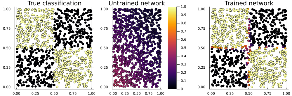
We’ll start from the XOR training example in the Flux.jl documentation. The trained network prediction plot is a great illustration of how well the network has learned the task. Here’s an example from a training run:
XOR Training Loss Surface
Clearly, the above training succeeded, as did the one in the original Flux.jl documentation. And there are longstanding claims that the XOR network loss surfaces for specific combinations of architecture, activation, and loss function have no local minima. But while experimenting with the code in the training example, I noticed that some of my trainings were getting stuck.
A Possible Cause
In reading about this phenomenon, I found this helpful summary, which I’ll quote in full:
The paper by Hamey cited in @LiKao’s answer proves there are no strict “regional local minima” for XOR in a 2-2-1 neural network. However, it admits “asymptotic minima” wherein the error surface flattens out as one or more weights approach infinity.
In practice, the weights don’t even need to be so large for this to happen and it is quite common for a 2-2-1 net to get stuck in this flat asymptotic region. The reason for this is saturation: the gradient of sigmoid activation approaches 0 as the weights get large, so the network is unable to keep learning.
See my notebook experiment - typically around 2 or 3 out of 10 networks end up stuck, even after 10,000 epochs. Results differ slightly if you change the learning rate, batch size, activation or loss functions, initial weights, whether inputs are created randomly or in a fixed order, etc. but usually a network gets stuck now and then.
The linked notebook is a reasonably compelling experiment, showing a mix of successful and stuck network trainings, with near zero gradients and relatively large weights for stuck ones.
Empirical Investigation
Let’s assume for the moment that the asymptotic minima claim is correct, and that there are wide, flat regions in the XOR loss surface for common small network configurations. What does it look like when training gets stuck? This is a 2-3-2 network, but it’s still pretty easy to induce for a fixed training set by varying the size of the network and choice of activation. I created a fixed XOR training set from the Flux.jl example code:
With this setup, the true and false cases are balanced:
sum(truth) / 10000.528If I were starting from scratch, I would probably do a setup more like the one from last post, where there’s a single 2x4 input example (which I might provide multiple times as a batch), but the approach here is fine as well.
I used this dataset to train various networks, including the one that produced the prediction plot above. I trained using my CPU for all of these examples, since they’re so small that there’s a large performance penalty when using a GPU, and it’s easier to ensure reproducibility in the CPU context.
Base Configuration (2-3-2 tanh)
Starting from the same 2-3-2 tanh network configuration as the Flux.jl docs, including batch normalization:
using Statistics, Plots

# Define our model, a multi-layer perceptron with one hidden layer of size 3:
model = Chain(
    Dense(2 => 3, tanh),   # activation function inside layer
    Dense(3 => 2, bias=false),
    softmax)

# The model encapsulates parameters, randomly initialised. Its initial output is:
out1 = model(noisy)                             # 2×1000 Matrix{Float32}

optim = Flux.setup(Flux.Adam(0.01), model);  # will store optimiser momentum, etc.

# Training loop, using the whole data set 1000 times:
function do_train!(model, optim, loader=loader, epochs=1e3)
    losses = []
    for epoch in 1:epochs
        for (x, y) in loader
            loss, grads = Flux.withgradient(model) do m
                # Evaluate model and loss inside gradient context:
                y_hat = m(x)
                Flux.crossentropy(y_hat, y)
            end
            Flux.update!(optim, model, grads[1])
            push!(losses, loss)  # logging, outside gradient context
        end
    end

    return losses
end

losses = do_train!(model, optim)

out2 = model(noisy)

function plot_predictions(noisy, truth, out1, out2)

    accuracy = mean((out2[1,:] .> 0.5) .== truth)

    p_true = scatter(noisy[1,:], noisy[2,:], zcolor=truth, title="True classification", legend=false)
    # p_raw =  scatter(noisy[1,:], noisy[2,:], zcolor=out1[1,:], title="Untrained network", label="", clims=(0,1))
    p_done = scatter(noisy[1,:], noisy[2,:], zcolor=out2[1,:], title="Trained network ($(accuracy))", legend=false)

    return plot(p_true, p_done, layout=(1,2)) # , size=(1000,330)

end

plot_predictions(noisy, truth, out1, out2)
This setup achieves 94% prediction accuracy, but has some areas of clear deficiency. I also don’t think batch normalization adds anything here, and I don’t believe in using it everywhere simply because it’s effective in some contexts. In fact, if we omit batch norm from the initial XOR network architecture, we can improve prediction accuracy on the same training dataset by 1.8%:
model = Chain(
    Dense(2 => 3, tanh),
    Dense(3 => 2, bias=false),
    softmax)

optim = Flux.setup(Flux.Adam(0.01), model)

losses = do_train!(model, optim)

plot_predictions(noisy, truth, out1, model(noisy))
We’d expect batch norm to help mitigate saturation, since it limits the magnitude of the weights; I’ll come back to that later. But as a starting point, I’ll take the 2-3-2 network above as the baseline. Given the fixed training dataset and random seed, we can easily induce failure in a couple of ways.
2-2-2 tanh
Removing one hidden node causes training to fail:
model = Chain(
    Dense(2 => 2, tanh),
    Dense(2 => 2, bias=false),
    softmax)
2-3-2 relu
Using the same network size and swapping in relu activation for tanh also results in training getting stuck:
model = Chain(
    Dense(2 => 3, relu),
    Dense(3 => 2, bias=false),
    softmax)
If activation saturation was the sole cause of stuck trainings, this network shouldn’t get stuck – relu doesn’t saturate; when the neuron output is above 0, it scales linearly to infinity.
2-3-2 celu
We can actually improve on the initial result by using the continuously differentiable exponential linear unit or celu in place of tanh or relu:
model = Chain(
    Dense(2 => 3, celu),
    Dense(3 => 2, bias=false),
    softmax)
celu doesn’t saturate either, like relu, but unlike relu, it’s smooth and has some gradient when the neuron output is below 0.
2-2-2 celu
But shrinking to 2 hidden nodes with the same setup results in even celu getting stuck:
model = Chain(
    Dense(2 => 2, celu),
    Dense(2 => 2, bias=false),
    softmax)
What About Batch Norm?
I repeated every experiment above both with and without batch norm. The training results were the same in terms of which networks got stuck and which didn’t, but for successful trainings, prediction accuracy was improved across the board without batch norm. I observed weights to top out at around 10 without batch norm, and around 1 with it, suggesting again that activation saturation isn’t the sole issue here.
Are These Trainings Really Stuck?
We can run the relu example for 5,000 epochs instead of 1,000, and plot the training loss:
model = Chain(
    Dense(2 => 3, relu),
    Dense(3 => 2, bias=false),
    softmax)
optim = Flux.setup(Flux.Adam(0.01), model)
losses = do_train!(model, optim, loader, 5e3)
plot(losses; xaxis=(:log10, "iteration"),
yaxis="loss", label="per batch")
n = length(loader)
plot!(n:n:length(losses), mean.(Iterators.partition(losses, n)),
label="epoch mean", dpi=200)In short, yes.
What About Other Seeds?
Perhaps I’ve just found a particularly intractable seed for this setup? I repeated the experiment with 10 seeds:
seeds = [8234, 6106, 7310, 1075, 2387, 4652, 157, 9614, 8439, 6105]
accuracies = []

for s in seeds

    Random.seed!(s)

    model = Chain(
        Dense(2 => 3, celu),
        Dense(3 => 2, bias=false),
    softmax)

    optim = Flux.setup(Flux.Adam(0.01), model)

    losses = do_train!(model, optim)

    accuracy = mean((model(noisy)[1,:] .> 0.5) .== truth)

    push!(accuracies, accuracy)

    @info "Seed $s, accuracy: $accuracy"

end

Random.seed!(359);
[ Info: Seed 8234, accuracy: 0.974
[ Info: Seed 6106, accuracy: 0.978
[ Info: Seed 7310, accuracy: 0.951
[ Info: Seed 1075, accuracy: 0.839
[ Info: Seed 2387, accuracy: 0.981
[ Info: Seed 4652, accuracy: 0.841
[ Info: Seed 157, accuracy: 0.979
[ Info: Seed 9614, accuracy: 0.84
[ Info: Seed 8439, accuracy: 0.979
[ Info: Seed 6105, accuracy: 0.975With the 2-3-2 celu setup that worked on our original seed, 3/10 trainings still get stuck at >10% accuracy below the rest.
What’s Going On Here?
I went looking for some more recent academic work on small neural network loss surfaces, particularly work exploring XOR networks. I found a series of papers from the same authors, with the most recent from summer 2023:
- Visualising Basins of Attraction for the Cross-Entropy and the Squared Error Neural Network Loss Functions
- Loss Surface Modality of Feed-Forward Neural Network Architectures
- Empirical Loss Landscape Analysis of Neural Network Activation Functions
The first one is lengthy, because it justifies and introduces a procedure for identifying basins of attraction in loss surfaces before applying it to explore the effects of loss function selection. The second and third papers are brief, since they apply the same procedure to compare architectures and activation functions.
Importantly, after recapping of prior work on the subject, all three papers show that the loss surface for small XOR networks has local minima across a range of examples. Training interacts with them differently depending on the architecture and activation.
The StackExchange post I linked previously, along with some of its references, cited activation saturation as the root cause here. The empirical activation paper agrees that saturation is an issue, but suggests that it can be mitigated with different choices of activation:
Bounded activation functions such as sigmoid and hyperbolic tangent (TanH) are prone to saturation, which was shown to be detrimental to NN performance for shallow [31] and deep [12] architectures alike. Modern activation functions such as rectified linear unit (ReLU) [27] and exponential linear unit (ELU) [7] are less prone to saturation, and thus became the primary choice for deep learning [1].
It’s certainly true that sigmoid and tanh are bounded whereas relu and the like are not. And yet in the above examples, we saw celu XOR networks get stuck in local minima in 3/10 example cases. The activation paper concludes:
Loss landscape modality, i.e. the total number of unique local minima, is not influenced by the choice of the activation function.
The choice of activation affects the shape of the loss landscape, particularly around its local minima, but not how many minima there are. To change that, as one of the conclusions from the network architectures paper claims:
An increase in the architecture width is shown to effectively reduce the number of local minima, and simplify the shape of the global attractor.
This is at least consistent with how we can induce training failures in the XOR procedure above by reducing the number of hidden nodes. And at a higher level, it’s consistent with broader findings about the effectiveness of overparameterized networks, which is a topic I might return to down the road.
Conclusions
There’s plenty more that could be unpacked here, which is an interesting thing to say about one of the simplest introductory neural network problems that exists. I think understanding XOR is a great way of building inuition about what makes neural networks effective.
The three loss landscape papers I cited above are also highly informative reads, and well worth perusing for anyone interested in thinking about what contributes to the success or failure of any given neural network training.
Other References
Post image courtesy of the Flux.jl project.